Tutorial 3 - Seasonality
Seasonality
Similar to prophet, judgyprophet models seasonality as Fourier series and can handle both additive and multiplicative seasonality. However, the seasonality implementation is currently limited to the index frequency and does not support the split into weekly, monthly, and yearly.
To enable seasonality, simply set the seasonal_period arg to a positive integer (e.g. 12 for monthly data, 7 for daily). The default seasonality is additive, to change this to multiplicative set the arg seasonal_type to be 'mult'. The Fourier order is set via the fourier_order parameter, with the default value set to seasonal_period - 1. The Fourier order determines how quickly the seasonality can change and the reducing order compared to the default parameters might help to avoid overfitting.
Additive Seasonality
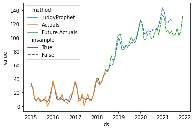
In the case of additive seasonality, the amplitude of the seasonal variation is independent of the trend and is hence roughly constant over the time series. If additive seasonality is selected, judgyprophet will rescale the time series onto zero mean and standard variance. An example is shown here:
from judgyprophet import JudgyProphet
import pandas as pd
import seaborn as sns
from judgyprophet.tutorials.resources import get_additive_seasonality_linear_trend

example_data = get_additive_seasonality_linear_trend()


# Cutoff the data to October 2020
cutoff = "2020-10-01"
data_cutoff = example_data.loc[:cutoff]

jp = JudgyProphet()
# We are passing in a simple time series without trend or level events. The seasonality is set to 12
#     and the seasonality component is simply additive.
jp.fit(
    data=data_cutoff,
    level_events=[],
    trend_events=[],
    seasonal_period=12,
    seasonal_type="add",
    # Set random seed for reproducibility
    seed=13
)
predictions = jp.predict(horizon=int(12))

# Plot the data:
predict_df = (
    predictions.reset_index()
    .rename(columns={'index': 'ds', 'forecast': 'value'})
    .assign(method="JudgyProphet")
    .loc[:, ["ds", "value", "insample", "method"]]
)
actuals_df = (
    data_cutoff.reset_index()
    .rename(columns={'index': 'ds', 0: 'value'})
    .assign(method="Actuals", insample=True)
)
future_actuals_df = (
    example_data.loc[cutoff:]
    .reset_index()
    .rename(columns={'index': 'ds', 0: 'value'})
    .assign(method="Future Actuals", insample=False)
)
plot_df = (
    pd.concat([predict_df, actuals_df, future_actuals_df])
    .reset_index(drop=True)
)

sns.lineplot(data=plot_df, x='ds', y='value', hue='method', style='insample', style_order=[True, False])
INFO:judgyprophet.judgyprophet:Rescaling onto 0-mean, 1-sd.
WARNING:judgyprophet.utils:No active trend or level events (i.e. no event indexes overlap with data). The model will just fit a base trend to the data.


Initial log joint probability = -891.479
    Iter      log prob        ||dx||      ||grad||       alpha      alpha0  # evals  Notes
      19      -1.34039   1.12595e-05    0.00168501      0.5461      0.5461       30
    Iter      log prob        ||dx||      ||grad||       alpha      alpha0  # evals  Notes
      21      -1.34039   1.01095e-06    0.00067455      0.1367      0.9362       33
Optimization terminated normally:
  Convergence detected: relative gradient magnitude is below tolerance


<AxesSubplot:xlabel='ds', ylabel='value'>
Multiplicative Seasonality
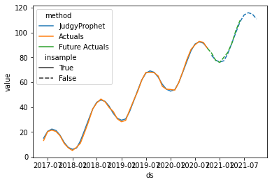
In case of multiplicative seasonality, the seasonal variations are changing proportional to the level of the series. If multiplicative seasonality is selected, judgyprophet will rescale the time series by shifting all values positive with standard variance. An example is shown here:
from judgyprophet import JudgyProphet
import pandas as pd
import seaborn as sns
from judgyprophet.tutorials.resources import get_multiplicative_seasonality_linear_trend

example_data = get_multiplicative_seasonality_linear_trend()


# Cutoff the data to October 2020
cutoff = "2020-10-01"
data_cutoff = example_data.loc[:cutoff]

jp = JudgyProphet()
# The multiplicative example time series has a constant trend component, but the seasonality
#     is multiplicative and has a large amplitude. Again the period is set to 12.
jp.fit(
    data=data_cutoff,
    level_events=[],
    trend_events=[],
    seasonal_period=12,
    seasonal_type="mult",
    # Set random seed for reproducibility
    seed=13
)
predictions = jp.predict(horizon=int(12))

# Plot the data:
predict_df = (
    predictions.reset_index()
    .rename(columns={'index': 'ds', 'forecast': 'value'})
    .assign(method="JudgyProphet")
    .loc[:, ["ds", "value", "insample", "method"]]
)
actuals_df = (
    data_cutoff.reset_index()
    .rename(columns={'index': 'ds', 0: 'value'})
    .assign(method="Actuals", insample=True)
)
future_actuals_df = (
    example_data.loc[cutoff:]
    .reset_index()
    .rename(columns={'index': 'ds', 0: 'value'})
    .assign(method="Future Actuals", insample=False)
)
plot_df = (
    pd.concat([predict_df, actuals_df, future_actuals_df])
    .reset_index(drop=True)
)

sns.lineplot(data=plot_df, x='ds', y='value', hue='method', style='insample', style_order=[True, False])
INFO:judgyprophet.judgyprophet:Rescaling by shifting all values positive with 1-sd.
WARNING:judgyprophet.utils:No active trend or level events (i.e. no event indexes overlap with data). The model will just fit a base trend to the data.


Initial log joint probability = -775.468
    Iter      log prob        ||dx||      ||grad||       alpha      alpha0  # evals  Notes
      19      -105.965     0.0490619       1203.53     0.04941           1       32
    Iter      log prob        ||dx||      ||grad||       alpha      alpha0  # evals  Notes
      39      -12.2029     0.0634662       440.207      0.1485      0.1485       64
    Iter      log prob        ||dx||      ||grad||       alpha      alpha0  # evals  Notes
      59     -0.683534     0.0372809       68.3501           1           1       84
    Iter      log prob        ||dx||      ||grad||       alpha      alpha0  # evals  Notes
      79     -0.454028    0.00336031       7.70556      0.8053      0.8053      109
    Iter      log prob        ||dx||      ||grad||       alpha      alpha0  # evals  Notes
      99     -0.442297   0.000894112       6.38619    0.006837           1      134
    Iter      log prob        ||dx||      ||grad||       alpha      alpha0  # evals  Notes
     119     -0.402061     0.0581892       7.15489      0.5184           1      159
    Iter      log prob        ||dx||      ||grad||       alpha      alpha0  # evals  Notes
     139     -0.287525     0.0223029      0.741186           1           1      187
    Iter      log prob        ||dx||      ||grad||       alpha      alpha0  # evals  Notes
     159     -0.285187   0.000493407       1.35585      0.3357           1      213
    Iter      log prob        ||dx||      ||grad||       alpha      alpha0  # evals  Notes
     179     -0.285081   5.78588e-05      0.106578      0.2866     0.02866      238
    Iter      log prob        ||dx||      ||grad||       alpha      alpha0  # evals  Notes
     199      -0.28508   6.70665e-06    0.00713309      0.1648      0.1648      259
    Iter      log prob        ||dx||      ||grad||       alpha      alpha0  # evals  Notes
     206      -0.28508   1.07542e-05    0.00613299           1           1      267
Optimization terminated normally:
  Convergence detected: relative gradient magnitude is below tolerance


<AxesSubplot:xlabel='ds', ylabel='value'>
Combining Seasonality with Events
Both seasonality can be combined with trend events, damping, level events, and unspecified changepoints. We will now walk through an example time series which contains a damped trend event and shows additive seasonality. Let's look at the data:
from judgyprophet.tutorials.resources import get_additive_seasonal_damped_trend_event

example_data = get_additive_seasonal_damped_trend_event()
example_data.plot.line()
<AxesSubplot:>
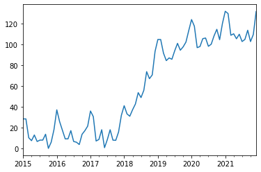
We can see from the plot that there is an uptick in trend around January 2018. The uptick in trend is quite steep until the end of 2019 where we observe stronger damping. We also see that the time series has a seasonal pattern, with a seasonal_period of 12 and a peak in December each year.
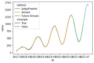
Forecasting with JudgyProphet before the event occurs
The estimate of the trend event is a trend increase of 6 with a damping parameter of 0.9.
from judgyprophet import JudgyProphet
import pandas as pd
import seaborn as sns

trend_events = [
    {'name': "New saturating market entry", 'index': '2018-01-01', 'm0': 6, 'gamma': .9}
]

# Cutoff the data to June 2017
cutoff = "2017-06-01"
data_cutoff = example_data.loc[:cutoff]

jp = JudgyProphet()
# We have one trend event and no level events. The seasonality is additive again.
jp.fit(
    data=data_cutoff,
    sigma_trend=0.1,
    level_events=[],
    unspecified_changepoints=10,
    sigma_unspecified_changepoints=.2,
    trend_events=trend_events,
    seasonal_period=12,
    seasonal_type="add",
    # Set random seed for reproducibility
    seed=13
)
predictions = jp.predict(horizon=int(36))

# Plot the data:
predict_df = (
    predictions.reset_index()
    .rename(columns={'index': 'ds', 'forecast': 'value'})
    .assign(method="JudgyProphet")
    .loc[:, ["ds", "value", "insample", "method"]]
)
actuals_df = (
    data_cutoff.reset_index()
    .rename(columns={'index': 'ds', 0: 'value'})
    .assign(method="Actuals", insample=True)
)
future_actuals_df = (
    example_data.loc[cutoff:]
    .reset_index()
    .rename(columns={'index': 'ds', 0: 'value'})
    .assign(method="Future Actuals", insample=False)
)
plot_df = (
    pd.concat([predict_df, actuals_df, future_actuals_df])
    .reset_index(drop=True)
)

sns.lineplot(data=plot_df, x='ds', y='value', hue='method', style='insample', style_order=[True, False])
INFO:judgyprophet.judgyprophet:Rescaling onto 0-mean, 1-sd.
WARNING:judgyprophet.judgyprophet:Post-event data for trend event New saturating market entry less than 0 points. Event deactivated in model. Event index: 2018-01-01, training data end index: 2015-01-01 00:00:00
WARNING:judgyprophet.utils:No active trend or level events (i.e. no event indexes overlap with data). The model will just fit a base trend to the data.


Initial log joint probability = -5618.69
    Iter      log prob        ||dx||      ||grad||       alpha      alpha0  # evals  Notes
      19      -19.5311      0.107624       53.5313           1           1       25
    Iter      log prob        ||dx||      ||grad||       alpha      alpha0  # evals  Notes
      39      -14.4873    0.00450173       32.1225           1           1       54
    Iter      log prob        ||dx||      ||grad||       alpha      alpha0  # evals  Notes
      59      -11.3416     0.0164259       63.5553      0.1261           1       83
    Iter      log prob        ||dx||      ||grad||       alpha      alpha0  # evals  Notes
      79       -10.031    0.00192964       42.0027      0.4045      0.4045      111
    Iter      log prob        ||dx||      ||grad||       alpha      alpha0  # evals  Notes
      99      -9.91568    0.00123052       20.6714      0.3407           1      136
    Iter      log prob        ||dx||      ||grad||       alpha      alpha0  # evals  Notes
     119      -9.74583     0.0178502       45.6554           1           1      161
    Iter      log prob        ||dx||      ||grad||       alpha      alpha0  # evals  Notes
     139      -9.58822    0.00240934       24.5607      0.1831           1      185
    Iter      log prob        ||dx||      ||grad||       alpha      alpha0  # evals  Notes
     159      -9.55939   0.000174537        18.265           1           1      214
    Iter      log prob        ||dx||      ||grad||       alpha      alpha0  # evals  Notes
     179      -9.55721   4.74996e-06       18.6232           1           1      243
    Iter      log prob        ||dx||      ||grad||       alpha      alpha0  # evals  Notes
     199      -9.55707   1.07478e-05       21.7289           1           1      267
    Iter      log prob        ||dx||      ||grad||       alpha      alpha0  # evals  Notes
     219       -9.5541    1.0315e-05       21.3723           1           1      288
    Iter      log prob        ||dx||      ||grad||       alpha      alpha0  # evals  Notes
     239      -9.50413    0.00075237       20.6816      0.6394      0.6394      309
    Iter      log prob        ||dx||      ||grad||       alpha      alpha0  # evals  Notes
     259      -9.41589   0.000411908       21.7004           1           1      331
    Iter      log prob        ||dx||      ||grad||       alpha      alpha0  # evals  Notes
     279      -9.39884   1.20103e-05       20.8879      0.3439      0.3439      355
    Iter      log prob        ||dx||      ||grad||       alpha      alpha0  # evals  Notes
     299      -9.39799   4.26641e-06       20.0502       0.476       0.476      379
    Iter      log prob        ||dx||      ||grad||       alpha      alpha0  # evals  Notes
     319      -9.37685   5.71275e-05        19.885      0.3824      0.3824      405
    Iter      log prob        ||dx||      ||grad||       alpha      alpha0  # evals  Notes
     339      -9.34918   0.000126588       18.6708      0.9182      0.9182      429
    Iter      log prob        ||dx||      ||grad||       alpha      alpha0  # evals  Notes
     359      -9.34728    1.3233e-05       20.7019           1           1      455
    Iter      log prob        ||dx||      ||grad||       alpha      alpha0  # evals  Notes
     379      -9.33447   2.78134e-05       20.1768      0.5231      0.5231      477
    Iter      log prob        ||dx||      ||grad||       alpha      alpha0  # evals  Notes
     399      -9.33284   2.29302e-06       20.0762      0.6157      0.6157      501
    Iter      log prob        ||dx||      ||grad||       alpha      alpha0  # evals  Notes
     419      -9.33248    1.2898e-05       19.1065     0.08486           1      529
    Iter      log prob        ||dx||      ||grad||       alpha      alpha0  # evals  Notes
     420      -9.33247   3.42574e-06       21.2674   1.793e-07       0.001      576  LS failed, Hessian reset
     439      -9.33237   2.57199e-07       22.0328      0.3448           1      603
    Iter      log prob        ||dx||      ||grad||       alpha      alpha0  # evals  Notes
     450      -9.33237   7.89272e-09       20.4987      0.2986           1      621
Optimization terminated normally:
  Convergence detected: absolute parameter change was below tolerance


<AxesSubplot:xlabel='ds', ylabel='value'>
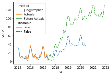
Forecasting with JudgyProphet after the event occurs
We can see that the model picks up correctly the seasonal pattern and incorporates the trend event. After a few more data points are observed, the model learned that the initial trend event estimates were poorly and corrects its forecast accordingly. Let's look at the forecast repeated in June 2018:
from judgyprophet import JudgyProphet
import pandas as pd
import seaborn as sns

trend_events = [
    {'name': "New saturating market entry", 'index': '2018-01-01', 'm0': 6, 'gamma': .9}
]

# Cutoff the data to June 2017
cutoff = "2018-06-01"
data_cutoff = example_data.loc[:cutoff]

jp = JudgyProphet()
# We have one trend event and no level events. The seasonality is additive again.
jp.fit(
    data=data_cutoff,
    sigma_trend=0.1,
    level_events=[],
    unspecified_changepoints=10,
    sigma_unspecified_changepoints=.2,
    trend_events=trend_events,
    seasonal_period=12,
    seasonal_type="add",
    # Set random seed for reproducibility
    seed=13
)
predictions = jp.predict(horizon=int(36))

# Plot the data:
predict_df = (
    predictions.reset_index()
    .rename(columns={'index': 'ds', 'forecast': 'value'})
    .assign(method="JudgyProphet")
    .loc[:, ["ds", "value", "insample", "method"]]
)
actuals_df = (
    data_cutoff.reset_index()
    .rename(columns={'index': 'ds', 0: 'value'})
    .assign(method="Actuals", insample=True)
)
future_actuals_df = (
    example_data.loc[cutoff:]
    .reset_index()
    .rename(columns={'index': 'ds', 0: 'value'})
    .assign(method="Future Actuals", insample=False)
)
plot_df = (
    pd.concat([predict_df, actuals_df, future_actuals_df])
    .reset_index(drop=True)
)

sns.lineplot(data=plot_df, x='ds', y='value', hue='method', style='insample', style_order=[True, False])
INFO:judgyprophet.judgyprophet:Rescaling onto 0-mean, 1-sd.
INFO:judgyprophet.judgyprophet:Adding trend event New saturating market entry to model. Event index: 2018-01-01, training data start index: 2015-01-01 00:00:00, training data end index: 2018-06-01 00:00:00. Initial gradient: 6. Damping: 0.9.
WARNING:judgyprophet.utils:Unspecified changepoint with index 2018-01-01 00:00:00 also specified as a level or trend event. Removing this changepoint.


Initial log joint probability = -4219.81
    Iter      log prob        ||dx||      ||grad||       alpha      alpha0  # evals  Notes
      19      -45.4011     0.0443425       326.047           1           1       26
    Iter      log prob        ||dx||      ||grad||       alpha      alpha0  # evals  Notes
      39      -15.3423    0.00201394       41.5814           1           1       53
    Iter      log prob        ||dx||      ||grad||       alpha      alpha0  # evals  Notes
      59      -11.4289     0.0222713       70.3068           1           1       82
    Iter      log prob        ||dx||      ||grad||       alpha      alpha0  # evals  Notes
      79      -9.74468     0.0019911       38.3992      0.8659      0.8659      110
    Iter      log prob        ||dx||      ||grad||       alpha      alpha0  # evals  Notes
      99      -9.55453    0.00466659       25.2859       0.949       0.949      137
    Iter      log prob        ||dx||      ||grad||       alpha      alpha0  # evals  Notes
     119      -9.42124   0.000328639       21.1329      0.3671           1      163
    Iter      log prob        ||dx||      ||grad||       alpha      alpha0  # evals  Notes
     139      -9.38936    0.00514148       27.2595           1           1      196
    Iter      log prob        ||dx||      ||grad||       alpha      alpha0  # evals  Notes
     159       -9.3399    0.00760439       37.8239           1           1      223
    Iter      log prob        ||dx||      ||grad||       alpha      alpha0  # evals  Notes
     179      -9.27552   0.000532321       24.6411      0.4927      0.4927      247
    Iter      log prob        ||dx||      ||grad||       alpha      alpha0  # evals  Notes
     199      -9.23377    0.00261612       16.9745      0.8399      0.8399      269
    Iter      log prob        ||dx||      ||grad||       alpha      alpha0  # evals  Notes
     202      -9.23013   0.000104263       18.2691   5.753e-06       0.001      364  LS failed, Hessian reset
     219      -9.19983    0.00127842       29.8317           1           1      381
    Iter      log prob        ||dx||      ||grad||       alpha      alpha0  # evals  Notes
     239      -9.16268    0.00026094       21.9496       3.298      0.3298      403
    Iter      log prob        ||dx||      ||grad||       alpha      alpha0  # evals  Notes
     259       -9.1381    0.00160896       29.4252      0.9121      0.9121      426
    Iter      log prob        ||dx||      ||grad||       alpha      alpha0  # evals  Notes
     279      -9.11448   0.000430079       17.2828           1           1      451
    Iter      log prob        ||dx||      ||grad||       alpha      alpha0  # evals  Notes
     299      -9.09913   0.000132984       15.3301      0.2225      0.2225      479
    Iter      log prob        ||dx||      ||grad||       alpha      alpha0  # evals  Notes
     319      -9.09577   7.96264e-05       20.5328      0.9646      0.9646      507
    Iter      log prob        ||dx||      ||grad||       alpha      alpha0  # evals  Notes
     339       -9.0927   5.35475e-06       18.2672        0.38           1      533
    Iter      log prob        ||dx||      ||grad||       alpha      alpha0  # evals  Notes
     359      -9.09266   1.83214e-08       16.0514           1           1      567
    Iter      log prob        ||dx||      ||grad||       alpha      alpha0  # evals  Notes
     365      -9.09266   6.04342e-09       18.2719      0.6683      0.6683      573
Optimization terminated normally:
  Convergence detected: absolute parameter change was below tolerance


/Users/kpxh622/github/judgyprophet/judgyprophet/utils.py:31: UserWarning: Unspecified changepoint with index 2018-01-01 00:00:00 also specified as a level or trend event. Removing this changepoint.
  warnings.warn(msg)


<AxesSubplot:xlabel='ds', ylabel='value'>