Tutorial 2 - Trend Events
Trend Events
In this tutorial we use judgyprophet to forecast a time series with a known/expected change in trend. This is called a trend_event and an example would be the following:
from judgyprophet.tutorials.resources import get_trend_event

example_data = get_trend_event()
example_data.plot.line()
<AxesSubplot:>
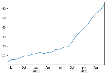
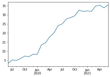
We can see from the plot that there is an uptick in trend around September 2020.
Format the trend event expectation for JudgyProphet
Suppose we are in April 2020, and we have the prior knowledge that an event will occur in September. The expected change of the trend gradient will be an uptick of 6. We can encode this in judgyprophet as an expected trend event as follows:
Each trend event is encoded as a dict with two required entries: the 'index' field, which is the index in the data when the event occurs. If this entry is fed into example_data.loc[], then it should return a single value. It follows the standard pandas indexing rules (for example, see here). The 'm0' field is the initial estimate by the business of what the impact of this event on the trend will be (e.g. in our case we estimate it will increase the trend by 6). It is fed into the model as an informative prior on the level event mean; which is then updated in a Bayesian way.
Forecasting with JudgyProphet before the event occurs
Now let's pretend we're still in April 2020, and see what judgyprophet would have forecasted:
from judgyprophet import JudgyProphet
import pandas as pd
import seaborn as sns

# Cutoff the data to January 2020
data_apr2020 = example_data.loc[:"2020-04-01"]

# Make the forecast with the business estimated level event
# We have no trend events, so just provide the empty list.
jp = JudgyProphet()
# Because the event is beyond the actuals, judgyprophet throws a warning.
#    This is just because the Bayesian model at the event has no actuals to learn from.
#    The event is still used in predictions.
jp.fit(
    data=data_apr2020,
    level_events=[],
    trend_events=trend_events,
    sigma_base_bias=1.,
    sigma_base_trend=1.,
    unspecified_changepoints=0,
    # Set random seed for reproducibility
    seed=13
)
predictions = jp.predict(horizon=12)
INFO:judgyprophet.judgyprophet:Rescaling onto 0-mean, 1-sd.
WARNING:judgyprophet.judgyprophet:Post-event data for trend event New market entry less than 0 points. Event deactivated in model. Event index: 2020-09-01, training data end index: 2019-06-01 00:00:00
WARNING:judgyprophet.utils:No active trend or level events (i.e. no event indexes overlap with data). The model will just fit a base trend to the data.


Initial log joint probability = -17.6559
    Iter      log prob        ||dx||      ||grad||       alpha      alpha0  # evals  Notes
       5      -2.70162    0.00625172   1.10466e-05           1           1        8
Optimization terminated normally:
  Convergence detected: relative gradient magnitude is below tolerance
Plotting the results:
predict_df = (
predictions.reset_index()
.rename(columns={'index': 'ds', 'forecast': 'value'})
.assign(method="JudgyProphet")
.loc[:, ["ds", "value", "insample", "method"]]
)
actuals_df = (
data_apr2020.reset_index()
.rename(columns={'index': 'ds', 0: 'value'})
.assign(method="Actuals", insample=True)
)
future_actuals_df = (
example_data.loc["2020-05-01":]
.reset_index()
.rename(columns={'index': 'ds', 0: 'value'})
.assign(method="Future Actuals", insample=False)
)
plot_df = (
pd.concat([predict_df, actuals_df, future_actuals_df])
.reset_index(drop=True)
)
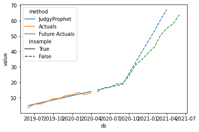
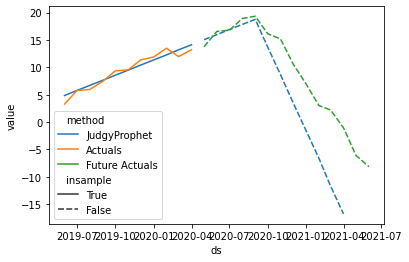
sns.lineplot(data=plot_df, x='ds', y='value', hue='method', style='insample', style_order=[True, False])
<AxesSubplot:xlabel='ds', ylabel='value'>
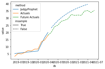
Forecasting with JudgyProphet after the event occurs
We can see that with the business information, the forecast is better able to handle the sudden uptick in trend. After a while though, we can see that the business estimate of the trend is an overestimate. Let's see if the Bayesian updating can account for this. We now suppose we are re-forecasting the product in January 2021.
from judgyprophet import JudgyProphet
import pandas as pd
import seaborn as sns

# Cutoff the data to January 2020
data_jan2021 = example_data.loc[:"2021-01-01"]

# Make the forecast with the business estimated level event
# We have no trend events, so just provide the empty list.
jp = JudgyProphet()
# Because the event is beyond the actuals, judgyprophet throws a warning.
#    This is just because the Bayesian model at the event has no actuals to learn from.
#    The event is still used in predictions.
jp.fit(
    data=data_jan2021,
    level_events=[],
    trend_events=trend_events,
    unspecified_changepoints=0,
    # Set random seed for reproducibility
    seed=13
)
predictions = jp.predict(horizon=12)
INFO:judgyprophet.judgyprophet:Rescaling onto 0-mean, 1-sd.
INFO:judgyprophet.judgyprophet:Adding trend event New market entry to model. Event index: 2020-09-01, training data start index: 2019-06-01 00:00:00, training data end index: 2021-01-01 00:00:00. Initial gradient: 6. Damping: None.


Initial log joint probability = -18.4007
    Iter      log prob        ||dx||      ||grad||       alpha      alpha0  # evals  Notes
       7      -1.64341   1.13818e-05   8.53133e-05           1           1       10
Optimization terminated normally:
  Convergence detected: relative gradient magnitude is below tolerance
predict_df = (
predictions.reset_index()
.rename(columns={'index': 'ds', 'forecast': 'value'})
.assign(method="JudgyProphet")
.loc[predictions.index <= "2021-06-01", ["ds", "value", "insample", "method"]]
)
actuals_df = (
data_apr2020.reset_index()
.rename(columns={'index': 'ds', 0: 'value'})
.assign(method="Actuals", insample=True)
)
future_actuals_df = (
example_data.loc["2020-05-01":]
.reset_index()
.rename(columns={'index': 'ds', 0: 'value'})
.assign(method="Future Actuals", insample=False)
)
plot_df = (
pd.concat([predict_df, actuals_df, future_actuals_df])
.reset_index(drop=True)
)
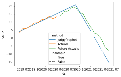
sns.lineplot(data=plot_df, x='ds', y='value', hue='method', style='insample', style_order=[True, False])
<AxesSubplot:xlabel='ds', ylabel='value'>
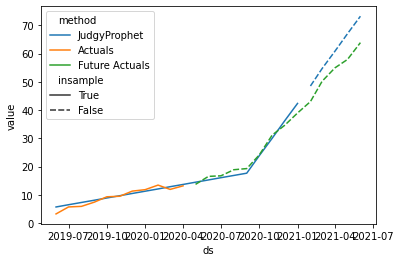
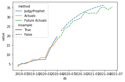
Although the forecast is still a slight overestimate, the Bayesian updating has downgraded the initial estimate somewhat.
Trend event reducing the historic trend
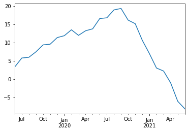
A trend event can also reduce the previous trend. A common real world examples for this case are a competitor entering the market and thus over time reducing your products market share.
<AxesSubplot:>
Format the trend event expectation for JudgyProphet
In this case, we simply add a minus to the expected trend impact:
Forecasting with JudgyProphet before the event occurs
Again, we're still in April 2020, and see what judgyprophet would have forecasted:
from judgyprophet import JudgyProphet
import pandas as pd
import seaborn as sns

# Cutoff the data to January 2020
data_apr2020 = example_data.loc[:"2020-04-01"]

# Make the forecast with the business estimated level event
# We have no trend events, so just provide the empty list.
jp = JudgyProphet()
# Because the event is beyond the actuals, judgyprophet throws a warning.
#    This is just because the Bayesian model at the event has no actuals to learn from.
#    The event is still used in predictions.
jp.fit(
    data=data_apr2020,
    level_events=[],
    trend_events=trend_events,
    sigma_base_bias=1.,
    sigma_base_trend=1.,
    unspecified_changepoints=0,
    # Set random seed for reproducibility
    seed=13
)
predictions = jp.predict(horizon=12)
INFO:judgyprophet.judgyprophet:Rescaling onto 0-mean, 1-sd.
WARNING:judgyprophet.judgyprophet:Post-event data for trend event New market entry less than 0 points. Event deactivated in model. Event index: 2020-09-01, training data end index: 2019-06-01 00:00:00
WARNING:judgyprophet.utils:No active trend or level events (i.e. no event indexes overlap with data). The model will just fit a base trend to the data.


Initial log joint probability = -3.20978
    Iter      log prob        ||dx||      ||grad||       alpha      alpha0  # evals  Notes
       7      -2.70162   5.03247e-05   6.65978e-05           1           1        9
Optimization terminated normally:
  Convergence detected: relative gradient magnitude is below tolerance
Plotting the results:
predict_df = (
predictions.reset_index()
.rename(columns={'index': 'ds', 'forecast': 'value'})
.assign(method="JudgyProphet")
.loc[:, ["ds", "value", "insample", "method"]]
)
actuals_df = (
data_apr2020.reset_index()
.rename(columns={'index': 'ds', 0: 'value'})
.assign(method="Actuals", insample=True)
)
future_actuals_df = (
example_data.loc["2020-05-01":]
.reset_index()
.rename(columns={'index': 'ds', 0: 'value'})
.assign(method="Future Actuals", insample=False)
)
plot_df = (
pd.concat([predict_df, actuals_df, future_actuals_df])
.reset_index(drop=True)
)
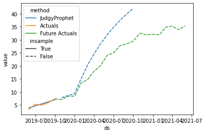
sns.lineplot(data=plot_df, x='ds', y='value', hue='method', style='insample', style_order=[True, False])
<AxesSubplot:xlabel='ds', ylabel='value'>
Forecasting with JudgyProphet after the event occurs
And after the event, we again learn from the additional data points:
from judgyprophet import JudgyProphet
import pandas as pd
import seaborn as sns

# Cutoff the data to January 2020
data_jan2021 = example_data.loc[:"2021-01-01"]

# Make the forecast with the business estimated level event
# We have no trend events, so just provide the empty list.
jp = JudgyProphet()
# Because the event is beyond the actuals, judgyprophet throws a warning.
#    This is just because the Bayesian model at the event has no actuals to learn from.
#    The event is still used in predictions.
jp.fit(
    data=data_jan2021,
    level_events=[],
    trend_events=trend_events,
    unspecified_changepoints=0,
    # Set random seed for reproducibility
    seed=13
)
predictions = jp.predict(horizon=12)
INFO:judgyprophet.judgyprophet:Rescaling onto 0-mean, 1-sd.
INFO:judgyprophet.judgyprophet:Adding trend event New market entry to model. Event index: 2020-09-01, training data start index: 2019-06-01 00:00:00, training data end index: 2021-01-01 00:00:00. Initial gradient: -6. Damping: None.


Initial log joint probability = -28.0997
    Iter      log prob        ||dx||      ||grad||       alpha      alpha0  # evals  Notes
       6      -7.46664   0.000740991   0.000446113           1           1        9
Optimization terminated normally:
  Convergence detected: relative gradient magnitude is below tolerance
predict_df = (
    predictions.reset_index()
    .rename(columns={'index': 'ds', 'forecast': 'value'})
    .assign(method="JudgyProphet")
    .loc[predictions.index <= "2021-06-01", ["ds", "value", "insample", "method"]]
)
actuals_df = (
    data_apr2020.reset_index()
    .rename(columns={'index': 'ds', 0: 'value'})
    .assign(method="Actuals", insample=True)
)
future_actuals_df = (
    example_data.loc["2020-05-01":]
    .reset_index()
    .rename(columns={'index': 'ds', 0: 'value'})
    .assign(method="Future Actuals", insample=False)
)
plot_df = (
    pd.concat([predict_df, actuals_df, future_actuals_df])
    .reset_index(drop=True)
)

sns.lineplot(data=plot_df, x='ds', y='value', hue='method', style='insample', style_order=[True, False])
<AxesSubplot:xlabel='ds', ylabel='value'>
Damping
In real world examples, we often observe that the initial trend after the event changes over time. A good example is the total sales of a product if this product is released to an additional new market. In this scenario, there is usually a period of strong uptake initially, followed by a slowing of uptake as the market saturates. We model this in judgyprophet by using damping. The damping model is a linear trend with damping, which is the same as that used in one of the most popular exponential smoothing methods: Holt's linear damped trend (see here).
Unlike the trend and level parameters, the damping is set by the user, and is not learnt during fitting. This is because we found learning using Bayesian fitting to be inaccurate. If you are not sure what the damping term should be we recommend using cross-validation, or observing similar market launches. The damping term is usually between 0.8 and 1 (where 1 means no damping, i.e. a linear model), it is equivalent to the $\phi$ parameter in the description of Holt's linear damped trend.
Those who know Prophet will remember it modelled this using logistic curves. We found this was extremely sensitive to the choice of the capacity parameter $C$ (the population the new entrant would eventually reach). This is why we opted for the damped linear trend, which we found to be more flexible.
Let's look at a curve with damping:
from judgyprophet.tutorials.resources import get_damped_trend_event

example_data = get_damped_trend_event()
print(example_data.head())
example_data.plot.line()
2019-06-01    3.287609
2019-07-01    5.253766
2019-08-01    4.955497
2019-09-01    5.951812
2019-10-01    7.345102
Freq: MS, dtype: float64


<AxesSubplot:>
We can see there is an initial uptick in trend, followed by a plateauing effect as the market saturates.
Format the damped trend event expectation for JudgyProphet
We talk to the business and they assume the initial trend uptake is 5, with a damping parameter from analysing similar market entrants of .9. We encode this as a trend_event as follows, notice that we refer to the damping parameter as gamma:
trend_events = [
    {'name': "New saturating market entry", 'index': '2020-01-01', 'm0': 5, 'gamma': .85}
]
Forecasting with JudgyProphet before the event occurs
from judgyprophet import JudgyProphet
import pandas as pd
import seaborn as sns

# Cutoff the data to January 2020
data_oct2019 = example_data.loc[:"2019-10-01"]

# Make the forecast with the business estimated level event
# We have no trend events, so just provide the empty list.
jp = JudgyProphet()
# Because the event is beyond the actuals, judgyprophet throws a warning.
#    This is just because the Bayesian model at the event has no actuals to learn from.
#    The event is still used in predictions.
jp.fit(
    data=data_oct2019,
    level_events=[],
    trend_events=trend_events,
    # Set random seed for reproducibility
    seed=13
)
predictions = jp.predict(horizon=12)

# Plot the data:
predict_df = (
    predictions.reset_index()
    .rename(columns={'index': 'ds', 'forecast': 'value'})
    .assign(method="JudgyProphet")
    .loc[:, ["ds", "value", "insample", "method"]]
)
actuals_df = (
    data_oct2019.reset_index()
    .rename(columns={'index': 'ds', 0: 'value'})
    .assign(method="Actuals", insample=True)
)
future_actuals_df = (
    example_data.loc["2019-10-01":]
    .reset_index()
    .rename(columns={'index': 'ds', 0: 'value'})
    .assign(method="Future Actuals", insample=False)
)
plot_df = (
    pd.concat([predict_df, actuals_df, future_actuals_df])
    .reset_index(drop=True)
)

sns.lineplot(data=plot_df, x='ds', y='value', hue='method', style='insample', style_order=[True, False])
WARNING:judgyprophet.utils:Arg 'data' has less than 5 data points. Expect a poor fit.
INFO:judgyprophet.judgyprophet:Rescaling onto 0-mean, 1-sd.
WARNING:judgyprophet.judgyprophet:Post-event data for trend event New saturating market entry less than 0 points. Event deactivated in model. Event index: 2020-01-01, training data end index: 2019-06-01 00:00:00
WARNING:judgyprophet.utils:No active trend or level events (i.e. no event indexes overlap with data). The model will just fit a base trend to the data.


Initial log joint probability = -4.75577
    Iter      log prob        ||dx||      ||grad||       alpha      alpha0  # evals  Notes
       4      -2.08579     0.0190169   7.99064e-06           1           1        6
Optimization terminated normally:
  Convergence detected: relative gradient magnitude is below tolerance


<AxesSubplot:xlabel='ds', ylabel='value'>
We can see the initial estimates are quite off this time. This is because the business overestimated the damping and the trend. Let's see what happens as we start to observe actuals.
Forecasting with JudgyProphet after the event occurs
from judgyprophet import JudgyProphet
import pandas as pd
import seaborn as sns

# Cutoff the data to January 2020
cutoff = "2020-04-01"
data_cutoff = example_data.loc[:cutoff]

# Make the forecast with the business estimated level event
# We have no trend events, so just provide the empty list.
jp = JudgyProphet()
# Because the event is beyond the actuals, judgyprophet throws a warning.
#    This is just because the Bayesian model at the event has no actuals to learn from.
#    The event is still used in predictions.
jp.fit(
    data=data_cutoff,
    level_events=[],
    trend_events=trend_events,
    # Set random seed for reproducibility
    seed=13
)
predictions = jp.predict(horizon=12)

# Plot the data:
predict_df = (
    predictions.reset_index()
    .rename(columns={'index': 'ds', 'forecast': 'value'})
    .assign(method="JudgyProphet")
    .loc[:, ["ds", "value", "insample", "method"]]
)
actuals_df = (
    data_cutoff.reset_index()
    .rename(columns={'index': 'ds', 0: 'value'})
    .assign(method="Actuals", insample=True)
)
future_actuals_df = (
    example_data.loc[cutoff:]
    .reset_index()
    .rename(columns={'index': 'ds', 0: 'value'})
    .assign(method="Future Actuals", insample=False)
)
plot_df = (
    pd.concat([predict_df, actuals_df, future_actuals_df])
    .reset_index(drop=True)
)

sns.lineplot(data=plot_df, x='ds', y='value', hue='method', style='insample', style_order=[True, False])
INFO:judgyprophet.judgyprophet:Rescaling onto 0-mean, 1-sd.
INFO:judgyprophet.judgyprophet:Adding trend event New saturating market entry to model. Event index: 2020-01-01, training data start index: 2019-06-01 00:00:00, training data end index: 2020-04-01 00:00:00. Initial gradient: 5. Damping: 0.85.


Initial log joint probability = -10.4473
    Iter      log prob        ||dx||      ||grad||       alpha      alpha0  # evals  Notes
       9      -2.49061   8.76664e-05    0.00143778      0.9171      0.9171       11
Optimization terminated normally:
  Convergence detected: relative gradient magnitude is below tolerance


<AxesSubplot:xlabel='ds', ylabel='value'>
While the trend is still a little overestimated, it is definitely improving. But is there anything we can do to improve the situation?
Unspecified Changepoints
Like prophet, we enable the user to include unspecified changepoints into the forecast. Unexpected changepoints enables us to handle unexpected changes in the trend of level of the time series. This is done by setting the unspecified_changepoints parameter in the fit method of JudgyProphet. Unspecified changepoints are initially set to have no effect on the model, but if actuals are observed that deviate from the model, they will be 'turned on,' and change the model.
The arg unspecified_changepoints either takes an integer as input, which will intersperse the changepoints equally across time, or a list of indexes, which will place changepoints at exactly those time points. These changepoints are given a Laplace prior with a mean of 0, and a scale set by the arg sigma_unspecified_changepoints. The sigma_unspecified_changepoints affects the L1 penalty on the unspecified changepoints. Set sigma to be high (e.g. .5 or greater) and the unspecified changepoints will be very sensitive. Set it low (e.g. 0.05), and it will be insensitive.
Unlike prophet, setting these changepoints does not change the prediction. Only level_events and trend_events in the prediction horizon will affect the forecast. Let's see what affect these have on the previous damping example...
from judgyprophet import JudgyProphet
import pandas as pd
import seaborn as sns

# Cutoff the data to January 2020
cutoff = "2020-04-01"
data_cutoff = example_data.loc[:cutoff]

# Make the forecast with the business estimated level event
# We have no trend events, so just provide the empty list.
jp = JudgyProphet()
# Because the event is beyond the actuals, judgyprophet throws a warning.
#    This is just because the Bayesian model at the event has no actuals to learn from.
#    The event is still used in predictions.
jp.fit(
    data=data_cutoff,
    level_events=[],
    unspecified_changepoints=10,
    sigma_unspecified_changepoints=.2,
    trend_events=trend_events,
    # Set random seed for reproducibility
    seed=13
)
predictions = jp.predict(horizon=12)

# Plot the data:
predict_df = (
    predictions.reset_index()
    .rename(columns={'index': 'ds', 'forecast': 'value'})
    .assign(method="JudgyProphet")
    .loc[:, ["ds", "value", "insample", "method"]]
)
actuals_df = (
    data_cutoff.reset_index()
    .rename(columns={'index': 'ds', 0: 'value'})
    .assign(method="Actuals", insample=True)
)
future_actuals_df = (
    example_data.loc[cutoff:]
    .reset_index()
    .rename(columns={'index': 'ds', 0: 'value'})
    .assign(method="Future Actuals", insample=False)
)
plot_df = (
    pd.concat([predict_df, actuals_df, future_actuals_df])
    .reset_index(drop=True)
)

sns.lineplot(data=plot_df, x='ds', y='value', hue='method', style='insample', style_order=[True, False])
INFO:judgyprophet.judgyprophet:Rescaling onto 0-mean, 1-sd.
INFO:judgyprophet.judgyprophet:Adding trend event New saturating market entry to model. Event index: 2020-01-01, training data start index: 2019-06-01 00:00:00, training data end index: 2020-04-01 00:00:00. Initial gradient: 5. Damping: 0.85.
WARNING:judgyprophet.utils:Unspecified changepoint with index 2020-01-01 00:00:00 also specified as a level or trend event. Removing this changepoint.


Initial log joint probability = -85.6424
    Iter      log prob        ||dx||      ||grad||       alpha      alpha0  # evals  Notes
      12      -2.55807    0.00253247       10.5928   0.0002553       0.001       57  LS failed, Hessian reset
      19      -2.53784    0.00129929       12.9114       2.828      0.4174       69
    Iter      log prob        ||dx||      ||grad||       alpha      alpha0  # evals  Notes
      39      -2.49159   1.88991e-05       13.7481     0.05264           1      106
    Iter      log prob        ||dx||      ||grad||       alpha      alpha0  # evals  Notes
      43      -2.49059   2.07785e-05        13.316   1.762e-06       0.001      150  LS failed, Hessian reset
      49      -2.48998    7.5683e-06       12.3042   6.778e-07       0.001      193  LS failed, Hessian reset
      59      -2.48991   3.40412e-07       12.2862      0.3482      0.3482      210
    Iter      log prob        ||dx||      ||grad||       alpha      alpha0  # evals  Notes
      70       -2.4899   8.88435e-09       11.2343   6.928e-10       0.001      271  LS failed, Hessian reset
Optimization terminated normally:
  Convergence detected: absolute parameter change was below tolerance


/Users/kpxh622/github/judgyprophet/judgyprophet/utils.py:31: UserWarning: Unspecified changepoint with index 2020-01-01 00:00:00 also specified as a level or trend event. Removing this changepoint.
  warnings.warn(msg)


<AxesSubplot:xlabel='ds', ylabel='value'>
We can see in this case the unspecified changepoints have improved the model fit significantly. We recommend caution with unspecified changepoints though, they come with a cost, and when your time series is quite noisy they might be overreactive. In this case it is recommended to tune your sigma_unspecified_changepoints accordingly, or limit the amount of changepoints you use.